Technical paper · Geophysical Log Workbench
Estimating formation-water salinity from geophysical logs
The resistivity–porosity method and the LCG TDS Estimator, with a Sedgwick well example from Thomas County, Georgia
A geophysical log is a record of formation and borehole response, not a direct measurement of groundwater salinity. Combining selected resistivity and porosity readings with a temperature estimate can nevertheless reveal a useful salinity profile when the geological assumptions are made explicit.
From log response to an interpreted salinity profile
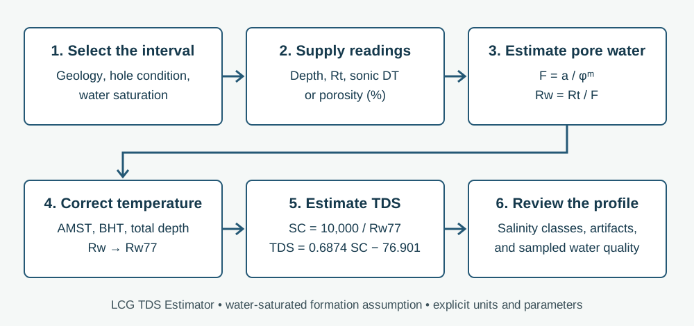
The Logic Cloud Geo (LCG) TDS Estimator implements a resistivity–porosity calculation for selected water-saturated intervals. The result is an estimate of formation-water total dissolved solids (TDS), in milligrams per liter (mg/L). It is a separate tool from the Well Log Plotter: the geologist selects representative readings, pastes three columns from a spreadsheet, reviews the temperature and formation assumptions, and examines the resulting depth profile.
The method is useful for locating salinity changes where sampled water-quality data are sparse. It does not replace a water sample, a borehole-condition review, or a geological interpretation. A continuous, automatically calculated TDS trace can contain artifacts; selected points and their surrounding log response should be examined together. This paper explains the calculation currently implemented in LCG and uses the GGS3114 Sedgwick well as its numerical reference.
Sources of data and preservation of lineage
The regional work that motivated this calculator drew on State-agency and USGS files: oil and gas test wells, deep injection wells, and test holes penetrating the brackish and saline parts of the Floridan and Southeastern Coastal Plain aquifer systems. Water-quality comparisons included produced-water analyses, interval-specific packer tests from injection-well reports, and USGS and water-management-district records with known completion intervals.
The author’s historical draft described 130 wells in Alabama, 747 in Florida, 304 in Georgia, 45 in South Carolina, and 21 offshore wells. Those figures describe an earlier inventory, not the present web application. The revised published DS760 record (Williams, Raines, and Lanning, 2016) reports 4,883 logs from 1,248 wells and organizes downloads by State and county. Scanned source logs, digitized LAS files, and wells used for interpretation are different populations and should not be counted interchangeably.
This paper adapts the author’s supplied internal methods narrative and figures. The numerical example comes from Table_02_Calc_FormationFactor.xls, worksheet TDS_FromLogs_Calc, rows 6–31. The accompanying salinity terminology comes from Table_01_SalinityZonesClasses.xls. These local source materials are distinguished from the published literature in the references; no placeholder USGS report number is treated as a publication.
Equations, units and assumptions
Archie’s formation-factor relationship connects the resistivity of a fully water-saturated formation, R₀, with that of its pore water, Rw. LCG accepts an interpreted true formation resistivity Rt from a suitable deep induction, long-normal, or other appropriate resistivity measurement and uses Rt as R₀ under the water-saturated assumption. The measured curve must be evaluated for invasion, borehole effects, lithology and tool response before making that substitution.
Porosity φ is a fraction in every equation below. If porosity is supplied in percent, LCG divides it by 100. In sonic mode the current example relation is φ = c(DT − DTma)/DT, with c = 0.625 and DTma = 49 µs/ft for the supplied Sedgwick workbook. This relation is not a universal sonic-porosity transform; its applicability must be justified for the formation being interpreted.
The dimensionless coefficient a and cementation exponent m describe the selected formation-factor relationship. They remain editable because texture, pore connectivity and carbonate complexity vary. LCG’s initial values a = 1.0 and m = 1.8 reproduce GGS3114; they are not statewide Florida defaults.
Formation temperature is estimated with a straight-line gradient from annual mean surface temperature (AMST) to bottom-hole temperature (BHT) at total depth (TD). Depth d and TD must use the same datum and feet. BHT and TD must describe the same temperature endpoint. A recorded logging temperature may differ from an equilibrated formation temperature, so the inferred gradient requires review.
After correcting water resistivity to 77°F (25°C), LCG converts it to specific conductance (SC, µS/cm). The implemented SC–TDS relationship, TDS = 0.6874 SC − 76.901, is the relationship in the supplied carbonate-well workbook. It is empirical and chemistry dependent. The historical sand-aquifer narrative also describes an approximate TDS = 0.67 SC relationship; that is a distinct conversion and is not the equation currently used by this calculator.
| Step | Equation | Units / qualification |
|---|---|---|
| Porosity from supplied values | φ = porosity (%) / 100 | fraction |
| Porosity from sonic (example) | φ = 0.625 × (DT − 49) / DT | DT in µs/ft |
| Formation factor | F = a / φᵐ | dimensionless |
| Formation-water resistivity | Rw = Rt / F | ohm-m; assumes Rt = R₀ |
| Formation temperature | Tf = AMST + (BHT − AMST) × d / TD | °F |
| Temperature normalization | Rw77 = Rw × (Tf + 6.77) / (77 + 6.77) | ohm-m at 77°F |
| Specific conductance | SC = 10,000 / Rw77 | µS/cm |
| Estimated dissolved solids | TDS = 0.6874 × SC − 76.901 | mg/L |
Worked example: GGS3114, I.E.W. Sedgwick No.1-A
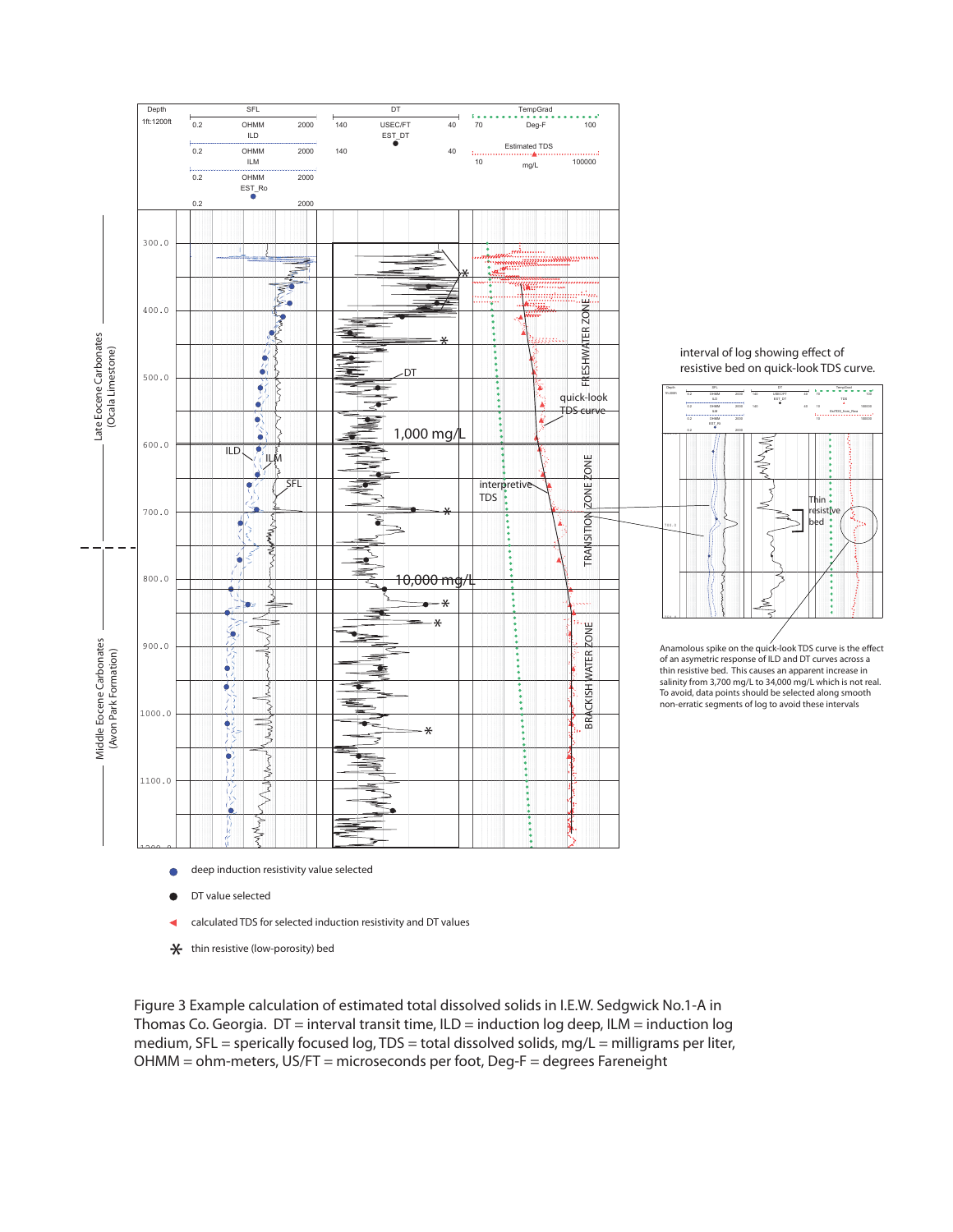
GGS3114 is the I.E.W. Sedgwick No.1-A well in Thomas County, Georgia, in the Thomasville area. The supplied log interpretation shows deep induction resistivity (ILD), shallower resistivity responses, a sonic interval-transit-time log (DT), selected readings, and an interpreted salinity profile. Decreasing deep resistivity through the approximately 600–750-ft interval helped focus the original analysis on the fresh-to-saline transition.
The example workbook uses AMST = 75°F, BHT = 148°F, TD = 6,668 ft, a = 1.0, m = 1.8, c = 0.625, and DTma = 49 µs/ft. A separate unused 70°F cell in the workbook is not the active AMST for the checked calculations. All 26 raw calculation rows have been independently reproduced, with maximum absolute TDS difference less than 0.0000001 mg/L before display rounding.
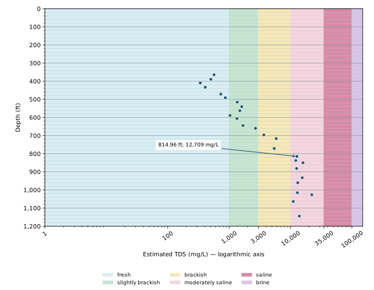
At d = 814.96 ft, Rt = 3.9637 ohm-m and DT = 98.9099 µs/ft yield porosity of about 31.54 percent and estimated TDS of approximately 12,709 mg/L. This is moderately saline water in the salinity transition zone under the supplied classification. The result represents the selected depth, not a sampled concentration or a precisely determined interface elevation.
The profile is not monotonic at every point. Thin resistive beds, mismatched vertical resolution, washouts, and unstable sonic response can create apparent salinity spikes. In the supplied figure, an apparent increase near a thin resistive bed is identified as a quick-look artifact. The geologist’s selection of representative intervals is therefore part of the method, rather than a cosmetic step after computation.
Salinity zones and classes
The supplied scheme, modified from Reese (1994, 2000) and Reese and Memberg (2000), groups six classes into five zones. The brackish-water zone spans the slightly brackish and brackish classes (1,000–10,000 mg/L). The salinity transition zone spans 10,000–35,000 mg/L. These terms describe interpreted salinity; they do not by themselves define water suitability or treatment requirements.
LCG explicitly assigns a shared class endpoint to the lower class: exactly 1,000 mg/L is fresh, 3,000 is slightly brackish, 10,000 is brackish, 35,000 is moderately saline, and 100,000 is saline. Brine is greater than 100,000 mg/L. This is a calculator convention resolving shared endpoints in the source table, not a newly attributed definition from Reese. Classification uses unrounded estimates.
The 10,000 mg/L surface has been used as a regional freshwater/saltwater-interface reference in Floridan mapping. A point profile helps bracket that concentration change, but points alone do not locate a continuous boundary or justify interpolation. The LCG chart therefore displays unconnected estimates and makes no automatic interface-depth calculation.
| Zone | Class | TDS |
|---|---|---|
| fresh water zone | fresh | 0 to 1,000 mg/L |
| brackish water zone | slightly brackish | 1,000 to 3,000 mg/L |
| brackish water zone | brackish | 3,000 to 10,000 mg/L |
| salinity transition zone | moderately saline | 10,000 to 35,000 mg/L |
| saline water zone | saline | 35,000 to 100,000 mg/L |
| brine water zone | brine | Greater than 100,000 mg/L |
A different interpretation task in sand aquifers
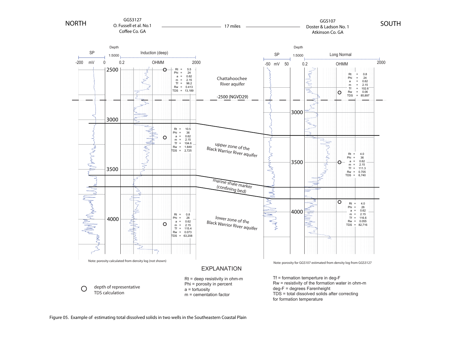
For the mostly sand aquifers of the Southeastern Coastal Plain, the original approach selected representative clean, low-clay beds. This reduced, but did not eliminate, the need to account for shaliness. In the supplied comparison of GGS3127 and GGS107, the interpretation follows the Chattahoochee River aquifer and upper and lower zones of the Black Warrior River aquifer. Where GGS107 lacked a porosity log, the original interpretation transferred porosity estimates from nearby GGS3127, about 17 miles away.
Such transferred porosity is an assumption that should be documented and tested. The historical comparison used a = 0.62 and m = 2.15, rather than the carbonate example’s a = 1.0 and m = 1.8. Neither set should be adopted merely because it appears in a worked figure. Clay conduction can invalidate a clean-formation Archie interpretation; Lee (2011), Simandoux (1963), Waxman and Smits (1968), and Worthington (1985) discuss aspects of that problem.
The historical comparison is retained as a qualitative illustration, not as a validation table. Some printed callouts do not reconcile: the GGS107 lower-zone callout lists Rt = 4.0 ohm-m, φ = 26 percent, a = 0.62 and m = 2.15, which imply uncorrected Rw ≈ 0.356 ohm-m, whereas the graphic prints 0.055. Those original callouts have not been silently revised. Use the reconciled GGS3114 rows to check the current calculator.
Using the calculator and reviewing the result
Select sonic DT in µs/ft or supplied porosity in percent. Copy Depth_ft, Rt_ohm_m and the matching third column from the example workbook or a prepared spreadsheet into the text box. The header is optional when data columns remain in that order. Review AMST, BHT, TD, a and m; in sonic mode, also review the sonic coefficient and matrix DT. Calculate only after the inputs describe the intended intervals.
The chart always begins at depth 0, with 100-ft major and 20-ft minor grid lines. The horizontal TDS axis is logarithmic. Pastel pink identifies moderately saline water and darker pink identifies saline water; class names and numerical results are also provided so color is not the only means of interpretation. Values below 1 mg/L appear only in the table. Negative estimates from the empirical relationship are retained for review and remain unclassified.
Review the detailed table as well as the chart. Changing an input clears the preceding results. Readings and calculations remain in the browser tab and are not uploaded to a personal archive. The table and figure are estimates conditional on the chosen relationship; no uncertainty bounds are calculated by the first release.
- Prefer representative, permeable, water-saturated intervals with stable log responses and compatible tool sampling depths.
- Inspect caliper and companion curves; avoid washouts, thin beds and obvious invasion or shale effects unless corrections are justified.
- Confirm the resistivity and sonic units, percent versus fractional porosity, temperature units, depths and datum.
- Compare estimates with interval-specific water samples where available and examine sensitivity to a, m, porosity and temperature.
- Do not interpret a salinity class as a laboratory analysis, a drinking-water determination, or a guaranteed treatment-resource boundary.
Source notes and reproducibility
The calculation table below includes all 26 rows from the raw calculation worksheet, including 1,026.51 ft, which is omitted from the supplied formatted Table 2. Displayed values are rounded; calculations and class assignments retain full precision. The original log and sand-aquifer comparison remain historical illustrations. Their original labels should be interpreted alongside the explicit current equations and salinity table in this paper.
The supplied equation sheet describes porosity as percent, but the reconciled formation-factor calculation uses fractional porosity. Its temperature-correction equation also labels the numerator R₀; the workbook calculation correctly uses formation-water resistivity Rw. This paper states the implemented notation explicitly. The coefficient pair 0.75 and 1.6 printed on that sheet is not the pair used by the GGS3114 workbook.
The historical draft’s Williams and Raines (2013) methods citation contains an unassigned report number. It is treated here as supplied unpublished project material, not as a completed Scientific Investigations Report. A related published contribution appears in the 2013 Georgia Water Resources Conference proceedings and is listed separately. The revised DS760 publication is cited using its 2016 edition.
| Depth (ft) | Rt (ohm-m) | DT (µs/ft) | Porosity (%) | F | Tf (°F) | Rw (ohm-m) | TDS (mg/L) |
|---|---|---|---|---|---|---|---|
| 364.5 | 333.263 | 63.8994 | 14.57 | 32.03 | 78.99 | 10.4035 | 568.5 |
| 389.3 | 285.655 | 67 | 16.79 | 24.82 | 79.26 | 11.5075 | 504.74 |
| 409.71 | 176.456 | 84.8637 | 26.41 | 10.98 | 79.49 | 16.0657 | 338.64 |
| 433.46 | 77.4477 | 126.164 | 38.23 | 5.65 | 79.75 | 13.7169 | 408.33 |
| 471.13 | 46.6907 | 125.115 | 38.02 | 5.7 | 80.16 | 8.1904 | 731.89 |
| 491.34 | 39.257 | 126.792 | 38.35 | 5.61 | 80.38 | 6.9923 | 868.07 |
| 515.35 | 33.6489 | 104.151 | 33.1 | 7.32 | 80.64 | 4.5979 | 1,355.85 |
| 540.42 | 28.842 | 103.522 | 32.92 | 7.39 | 80.92 | 3.9028 | 1,605.72 |
| 562.6 | 27.2221 | 112.327 | 35.24 | 6.54 | 81.16 | 4.1638 | 1,495.89 |
| 588.58 | 33.6489 | 124.486 | 37.9 | 5.73 | 81.44 | 5.8681 | 1,035.51 |
| 606.3 | 29.9752 | 112.327 | 35.24 | 6.54 | 81.64 | 4.585 | 1,343.7 |
| 644.49 | 27.2221 | 103.522 | 32.92 | 7.39 | 82.06 | 3.6836 | 1,682.98 |
| 659.84 | 14.9798 | 114.004 | 35.64 | 6.41 | 82.22 | 2.3384 | 2,690.12 |
| 696.39 | 25.6931 | 76.0587 | 22.24 | 14.97 | 82.62 | 1.7159 | 3,677.19 |
| 716.54 | 7.9315 | 104.151 | 33.1 | 7.32 | 82.84 | 1.0838 | 5,852.04 |
| 771.26 | 7.486 | 113.375 | 35.49 | 6.45 | 83.44 | 1.1598 | 5,426.49 |
| 814.96 | 3.9637 | 98.9099 | 31.54 | 7.98 | 83.92 | 0.4966 | 12,709.24 |
| 837.86 | 13.604 | 66.2055 | 16.24 | 26.35 | 84.17 | 0.5162 | 12,188.66 |
| 850 | 3.0265 | 101.216 | 32.24 | 7.67 | 84.31 | 0.3946 | 15,946.97 |
| 881.43 | 2.9 | 122.809 | 37.56 | 5.83 | 84.65 | 0.4977 | 12,579.02 |
| 932.68 | 3.0265 | 102.264 | 32.55 | 7.54 | 85.21 | 0.4014 | 15,518.29 |
| 960.17 | 2.8566 | 119.245 | 36.82 | 6.04 | 85.51 | 0.4729 | 13,119.06 |
| 1,015.03 | 3.0265 | 114.633 | 35.78 | 6.36 | 86.11 | 0.476 | 12,947.92 |
| 1,026.51 | 5.395 | 70.8176 | 19.26 | 19.4 | 86.24 | 0.2781 | 22,187.08 |
| 1,063.52 | 3.3326 | 119.245 | 36.82 | 6.04 | 86.64 | 0.5517 | 11,096.96 |
| 1,144.42 | 3.9637 | 92.4109 | 29.36 | 9.08 | 87.53 | 0.4366 | 13,910.29 |
Selected references and supplied materials
- Archie, G.E., 1942, The electrical resistivity log as an aid in determining some reservoir characteristics: Transactions of the AIME, v. 146, p. 54–62.
- Asquith, G., and Krygowski, D., 2004, Basic Well Log Analysis, 2nd ed.: AAPG Methods in Exploration, no. 16.
- Lee, M.W., 2011, Connection equation and shaly-sand correction for electrical resistivity: USGS Scientific Investigations Report 2011–5005.
- Reese, R.S., 1994, Hydrogeology and the distribution and origin of salinity in the Floridan aquifer system, southeastern Florida: USGS Water-Resources Investigations Report 94–4010.
- Reese, R.S., 2000, Hydrogeology and the distribution of salinity in the Floridan aquifer system, southwestern Florida: USGS Water-Resources Investigations Report 98–4253.
- Reese, R.S., and Memberg, S.J., 2000, Hydrogeology and the distribution of salinity in the Floridan aquifer system, Palm Beach County, Florida: USGS Water-Resources Investigations Report 99–4061.
- Simandoux, P., 1963, Dielectric measurements on porous media: application to measurement of water saturations: Revue de l’Institut Français du Pétrole, v. 18, supplementary issue, p. 193–215.
- Waxman, M.H., and Smits, L.J.M., 1968, Electrical conductivities in oil-bearing shaly sands: Society of Petroleum Engineers Journal, v. 8, p. 107–122.
- Worthington, P.F., 1985, The evolution of shaly-sand concepts in reservoir evaluation: The Log Analyst, January–February, p. 23–40.
- Williams, L.J., and Raines, J.E., 2013, Using conventional borehole geophysical logs to map salinity variations in carbonate rock aquifer systems: Proceedings of the 2013 Georgia Water Resources Conference.
- Williams, L.J., Raines, J.E., and Lanning, A.E., 2016, Geophysical log database for the Floridan aquifer system and southeastern Coastal Plain aquifer system in Florida and parts of Georgia, Alabama, and South Carolina: USGS Data Series 760 (revised edition).
- Williams, L.J., supplied project materials: internal salinity-methods narrative; Sedgwick log interpretation; Southeastern Coastal Plain comparison; equation sheet; Table_02_Calc_FormationFactor.xls; and Table_01_SalinityZonesClasses.xls. Unpublished materials supplied for this LCG implementation.